Arrhenius Equation & Activation Energy Guide: 2-Temp Solving, Plots & Half-Lives

Whether you are solving a physical chemistry homework problem where activation energy $E_a$ suddenly came out off by a factor of 1,000, trying to verify a four-point $\mathrm{N_2O_5}$ Arrhenius plot slope and Eyring transition-state parameters ($\Delta H^\ddagger, \Delta S^\ddagger, \Delta G^\ddagger$) for a lab report, or predicting half-life ($t_{1/2}$) and 90% shelf-life ($t_{90}$) in accelerated stability testing, almost every kinetics error boils down to four traps: leaving °C instead of Kelvin, mixing kJ/mol with J/(mol·K), dividing by 2.303 vs natural log, or flipping $(1/T_1 - 1/T_2)$.

This guide gives you a single reference table for all key kinetics equations, explains when to choose CODATA vs textbook $R$, walks through five independently verified worked examples (with clickable pre-filled links into the Arrhenius Equation & Reaction Rate Calculator), and outlines when simple Arrhenius linearity breaks down.

Quick Reference: Essential Arrhenius, Eyring & Integrated Rate Equations

Gas Constant $R$: CODATA Exact Value vs Rounded Textbook Values

Small trailing-digit mismatches between your calculator and an answer key usually trace back to which standard value of the molar gas constant $R$ was used:

For a reaction whose rate exactly doubles between $25.0^\circ\text{C}$ and $35.0^\circ\text{C}$, exact CODATA $R$ yields $52.95\text{ kJ/mol}$, whereas rounded $R = 8.31$ yields $52.92\text{ kJ/mol}$ (~0.054% difference). You can toggle between both modes directly inside the Arrhenius Calculator.

Visual Guide: Arrhenius Slope ($-E_a/R$) & Half-Life Decay by Reaction Order

Understanding the geometry of both graphs prevents almost every conceptual error in chemical kinetics:

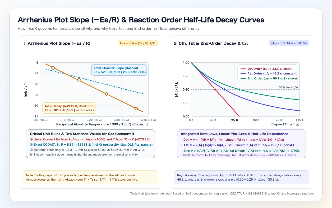
On the left panel, because the x-axis plots reciprocal temperature $1000/T$, hotter conditions sit on the left and cooler conditions sit on the right. A steeper negative slope indicates a higher activation energy $E_a$—meaning reaction rate rises sharply per 10 °C increase.

On the right panel, all three reaction orders begin at $[A]_0 = 1.00\text{ M}$ with numerically identical $k = 0.0150$:

• Zero-order falls in a straight line ($t_{1/2} = 33.3\text{ s}$) and hits zero completely at $66.67\text{ s}$.
• First-order decays exponentially with constant $t_{1/2} = 46.2\text{ s}$.
• Second-order reaches $50\%$ at $t_{1/2} = 66.7\text{ s}$, then slows dramatically because remaining molecules collide less often—taking $133.3\text{ s}$ just to go from $0.50\text{ M} \to 0.25\text{ M}$.

Five Worked Examples (With One-Click Calculator Pre-Fill Links)

Example 1: Solving $E_a$ from Two Temperatures (The “+10 °C Rate Doubles” Rule)

Problem: A reaction doubles its rate constant ($k_2 / k_1 = 2.00$) when warmed from $25.0^\circ\text{C}$ to $35.0^\circ\text{C}$. Find $E_a$ in $\text{kJ/mol}$ using CODATA $R = 8.3144626\text{ J/(mol}\cdot\text{K)}$.

1. Convert temperatures to Kelvin: $T_1 = 298.15\text{ K}$, $T_2 = 308.15\text{ K}$.
2. Compute reciprocal difference: $\frac{1}{298.15} - \frac{1}{308.15} = 1.088437 \times 10^{-4}\ \text{K}^{-1}$.
3. Solve for $E_a$: $E_a = \frac{8.3144626 \times \ln(2.00)}{1.088437 \times 10^{-4}} \approx 52,953.5\text{ J/mol} = \mathbf{52.95\text{ kJ/mol}}$

This explains why the classic rule of thumb (“reaction rates double every 10 °C near room temperature”, $Q_{10} \approx 2$) corresponds specifically to reactions with $E_a \approx 53\text{ kJ/mol}$.

👉 Load Example 1 into the Arrhenius Calculator to Verify

Example 2: Predicting Rate Constant $k_2$ at Higher Temperature ($\mathrm{N_2O_5}$ Decay)

Problem: For $\mathrm{N_2O_5}$ decomposition, $E_a = 103.0\text{ kJ/mol}$ and $k_1 = 3.46 \times 10^{-5}\text{ s}^{-1}$ at $25.0^\circ\text{C}$. Predict $k_2$ at $45.0^\circ\text{C}$.

1. Convert units: $E_a = 103,000\text{ J/mol}$, $T_1 = 298.15\text{ K}$, $T_2 = 318.15\text{ K}$.
2. Compute log ratio: $\ln\!\left(\frac{k_2}{k_1}\right) = \frac{103,000}{8.3144626}\left(\frac{1}{298.15} - \frac{1}{318.15}\right) = 2.61197$
3. Exponentiate and multiply: $\frac{k_2}{k_1} = e^{2.61197} \approx \mathbf{13.63\times}, \qquad k_2 = 13.6258 \times 3.46 \times 10^{-5} \approx \mathbf{4.71 \times 10^{-4}\text{ s}^{-1}}$

👉 Load Example 2 (N₂O₅ 25°C → 45°C Prediction) into the Calculator

Example 3: Finding Target Temperature $T_2$ for a 10× Speedup

Problem: A process has $E_a = 80.0\text{ kJ/mol}$. Starting at $27.0^\circ\text{C}$ ($300.15\text{ K}$), what temperature $T_2$ makes the reaction 10.0 times faster?

1. Rearrange for $1/T_2$: $\frac{1}{T_2} = \frac{1}{300.15} - \frac{8.3144626 \times \ln(10.0)}{80,000} = 3.092358 \times 10^{-3}\ \text{K}^{-1}$
2. Invert and convert back to Celsius: $T_2 = 323.38\text{ K} \implies \mathbf{50.23^\circ\text{C}}$

👉 Load Example 3 (Target Temperature for 10× Rate) into the Calculator

Example 4: Multi-Point OLS Arrhenius Plot & Eyring Transition-State Analysis

Dataset ($\mathrm{N_2O_5}$ decomposition across 4 temperatures):
(25.0 °C, 3.46e-5 s⁻¹), (35.0 °C, 1.35e-4 s⁻¹), (45.0 °C, 4.98e-4 s⁻¹), (55.0 °C, 1.50e-3 s⁻¹)

Running ordinary least-squares regression of $\ln k$ vs $1/T$ across all four points gives:

• Activation Energy: $E_a = \mathbf{102.68 \pm 1.54\text{ kJ/mol}}$ ($R^2 = 0.9996$)
• Pre-exponential Factor: $A = \mathbf{3.42 \times 10^{13}\text{ s}^{-1}}$
• Eyring Enthalpy of Activation at 25.0 °C: $\Delta H^\ddagger = E_a - R T_{\text{ref}} \approx \mathbf{+100.20\text{ kJ/mol}}$

If you want to review the underlying regression formulas for slope confidence intervals and $R^2$, see our Least Squares Linear Regression Guide.

👉 Load Example 4 (4-Point Arrhenius Plot & Eyring Fit) into the Calculator

Example 5: Integrated First-Order Decay, Half-Life $t_{1/2}$, and Shelf-Life $t_{90}$

Problem: Given $[A]_0 = 1.00\text{ M}$ and first-order $k = 0.0150\text{ s}^{-1}$, compute $[A]_t$ after $60.0\text{ s}$, half-life $t_{1/2}$, and $t_{90}$ (time for 10% loss).

• Remaining concentration: $[A]_{60} = 1.00 \times e^{-0.0150 \times 60.0} = \mathbf{0.4066\text{ M}}\ (40.66\%)$
• Half-life: $t_{1/2} = \frac{\ln 2}{0.0150} = \mathbf{46.21\text{ s}}$
• 90% remaining time ($t_{90}$): $t_{90} = \frac{-\ln 0.90}{0.0150} = \mathbf{7.024\text{ s}}$

👉 Load Example 5 (First-Order Decay, t₁/₂ & t₉₀) into the Calculator

Common Mistakes & Physical Limits of Ideal Arrhenius Kinetics

Four Mistakes to Double-Check Before Submitting

1. Using Celsius directly: Never write $1/25 - 1/35$; always convert to Kelvin first.
2. Factor-of-1,000 unit mismatch: Remember most organic/inorganic reactions sit in the $20 \text{ to } 200\text{ kJ/mol}$ range. Getting $53\text{ J/mol}$ or $53,000\text{ kJ/mol}$ almost always means you forgot $\times 1000$.
3. Using base-10 log (LOG10) in spreadsheets with -R: If your sheet computes $\log_{10} k$ instead of natural log $\ln k$, multiplying slope by $-R$ underestimates $E_a$ by $\ln(10) \approx 2.3026$. Always use LN(k).
4. Assuming every half-life stays constant: Only 1st-order decay keeps constant $t_{1/2}$; 0th- and 2nd-order half-lives shift as concentration changes.

When Real Systems Deviate from Linear Arrhenius Behavior

• Quantum tunneling & temperature-dependent $\Delta C_p^\ddagger$: Over wide temperature spans or light-atom proton transfers at low $T$, plots of $\ln k$ vs $1/T$ curve noticeably.
• Enzyme denaturation & phase changes: Biological catalysts lose activity abruptly above denaturation temperatures, producing sharp downward breaks on the high-temperature side (left side of the plot).
• Multi-step mechanisms: When the rate-determining step shifts with temperature, the fitted slope represents an apparent activation energy rather than a single elementary transition barrier.

Related Calculators & Further Reading

• Arrhenius Equation & Reaction Kinetics Calculator — Interactive two-temperature solver, multi-point OLS Arrhenius/Eyring analyzer, and 0th/1st/2nd-order decay tool.
• Least Squares Regression Calculator & Regression Guide — Detailed linear fitting, residuals, and $R^2$ checks.
• Natural & Common Logarithm Calculator & Logarithms Guide — Quick checks on $\ln$ vs $\log_{10}$ conversions.
• Half-Life Calculator & Half-Life Guide — Extended exponential decay workflows.
• Bond Energy & Enthalpy Calculator — Estimate reaction $\Delta H$ alongside kinetic barriers.

References

• IUPAC Compendium of Chemical Terminology (Gold Book) — Arrhenius equation (A00446) International standard definition of the Arrhenius equation and pre-exponential factor $A$.
• IUPAC Compendium of Chemical Terminology (Gold Book) — Activation energy (A00102) Formal empirical definition $E_a = RT^2\,\mathrm{d}(\ln k)/\mathrm{d}T$.
• NIST CODATA 2022 — Molar Gas Constant R Exact SI value of the molar gas constant ($R = 8.314\,462\,618\dots\text{ J mol}^{-1}\text{ K}^{-1}$).
• OpenStax Chemistry 2e — Section 12.5: Collision Theory & Arrhenius Equation Standard derivation of collision theory, activation barriers, and two-temperature Arrhenius plotting.
• OpenStax Chemistry 2e — Section 12.4: Integrated Rate Laws & Half-Life Derivation of 0th-, 1st-, and 2nd-order integrated rate equations and half-life dependencies.