When analyzing UV-Vis spectrophotometry data for a chemistry or biochemistry lab report, three mistakes account for most calculation errors: forgetting to convert μmol/L or mmol/L to mol/L before dividing by ε, using 1.0 cm instead of 0.10 cm for a 1.0 mm microvolume path length, and omitting the dilution factor (DF) when converting cuvette concentration back to the original sample concentration in mg/L (ppm).
This guide walks through 1) solving A = εcℓ in any direction with unit and dilution conversions, 2) converting between percent transmittance (%T), dark-corrected intensity, and absorbance A, and 3) fitting a 5-point least-squares calibration curve to quantify an unknown sample, alongside exact verification steps in the Beer-Lambert Law, Absorbance & Calibration Calculator. All numerical examples below are educational calculation models rather than certified measurements of a specific instrument.
Which Formula Should You Use? Quick Reference Table
First, match what you want to find with the required base units. Whenever molar absorptivity ε is given in L/(mol·cm) (equivalent to M⁻¹·cm⁻¹), concentration c must be in mol/L and path length ℓ must be in cm.
| Target Quantity | Required Inputs & Base Units | Formula | Calculator Tab & Mode |
|---|---|---|---|
| Absorbance A | ε [L/(mol·cm)], c [mol/L], ℓ [cm] | A = ε · c · ℓ | Tab 1 (A = εcℓ Solver) → Solve for Absorbance A |
| Cuvette Molarity c | A [AU], ε [L/(mol·cm)], ℓ [cm] | c = A / (ε · ℓ) | Tab 1 (A = εcℓ Solver) → Solve for Concentration c |
| Molar Absorptivity ε | A [AU], c [mol/L], ℓ [cm] | ε = A / (c · ℓ) | Tab 1 (A = εcℓ Solver) → Solve for Molar Absorptivity ε |
| Undiluted Stock c₀ & Mass Conc. ρ₀ | Cuvette c, Dilution Factor DF, Molar Mass M [g/mol] | c₀ = c × DF, ρ₀ [mg/L] = c₀ [mol/L] × M × 1000 | Tab 1 lower fields (Dilution Factor DF, Molar Mass M) |
| Transmittance %T ⇄ Absorbance A | %T [%] or Intensities I₀, I, I_dark | T = (I − I_dark)/(I₀ − I_dark), A = −log₁₀T = 2 − log₁₀(%T) | Tab 2 (Absorbance A ⇄ %T & Intensity) |
| Calibration Curve & Unknown c | Standards (cᵢ, Aᵢ), Unknown A_sample, DF | A = m·c + b, c_unknown = (A_sample − b)/m, c₀ = c_unknown × DF | Tab 3 (Calibration Curve & Unknowns) |
Although absorbance A is strictly dimensionless, it is commonly reported with the suffix AU (Absorbance Units) or Abs in laboratory documentation to distinguish it from transmittance or raw detector counts.
Example 1: Finding Absorbance of NADH at 340 nm (Converting μmol/L to mol/L)
Suppose an enzymatic assay solution contains NADH at a cuvette concentration of c = 50 μmol/L in a standard ℓ = 1.0 cm cuvette, with molar absorptivity ε = 6220 L/(mol·cm) at 340 nm.
- Convert concentration to mol/L: Since 1 μmol/L = 10⁻⁶ mol/L, c = 50 × 10⁻⁶ = 5.0 × 10⁻⁵ mol/L.
- Calculate absorbance A:
- Convert to transmittance ratio T and %T:
- Fraction of light absorbed: 100% − 48.87% = 51.13%.
Multiplying 6220 × 50 × 1.0 = 311,000 without converting μmol/L to mol/L is the single most common unit error in Beer-Lambert problems.
Example 2: Back-Calculating Unknown Concentration with Dilution Factor (DF) and mg/L
Suppose a potassium permanganate (KMnO₄, molar mass M = 158.034 g/mol) stock solution was too concentrated to read directly, so you diluted it 10-fold (e.g., 10 mL stock diluted to 100 mL total volume, DF = 10). At 525 nm (ε = 2455 L/(mol·cm), ℓ = 1.0 cm), the diluted solution gives an absorbance of A = 0.491 AU.
| Step | Substitution & Formula | Result |
|---|---|---|
| 1. Diluted cuvette molarity c | c = 0.491 ÷ (2455 × 1.0) | 0.0002000 mol/L = 200.0 μmol/L (0.2000 mmol/L) |
| 2. Undiluted stock molarity c₀ | c₀ = c × DF = 200.0 μmol/L × 10 | 2000 μmol/L = 2.000 mmol/L (0.002000 mol/L) |
| 3. Stock mass concentration ρ₀ (mg/L) | ρ₀ = 0.002000 mol/L × 158.034 g/mol × 1000 mg/g | 316.07 mg/L (approx. 316.07 ppm in dilute aqueous solution) |
For preparing standard dilutions using C₁V₁ = C₂V₂, see the Molarity and Dilution Calculation Guide and the Dilution Calculator.
Microvolume Spectrophotometers (Path Length ℓ = 1.0 mm = 0.10 cm)
Microvolume UV-Vis instruments used for nucleic acids (dsDNA at 260 nm) and proteins often measure across a 1.0 mm (0.10 cm) or 0.5 mm gap rather than a 1.0 cm cuvette.
For example, if dsDNA (average nucleotide molar absorptivity ε = 6600 L/(mol·cm), average nucleotide molar mass M = 330 g/mol) shows a raw absorbance of A = 0.150 AU across a ℓ = 1.0 mm = 0.10 cm path length (equivalent to 1.50 AU at 1.0 cm):
Entering ℓ = 1.0 cm by mistake yields 22.73 μmol/L—off by a factor of 10. Always check whether your instrument software exports the raw absorbance at the actual gap length or an absorbance already normalized to 10 mm (1.0 cm).
Example 3: Transmittance %T, Dark-Signal Subtraction, and High-Absorbance Stray Light
A spectrophotometer compares the radiant power transmitted through a blank (I₀) with the power transmitted through the sample (I), subtracting any detector dark signal (I_dark) measured when the beam is blocked:
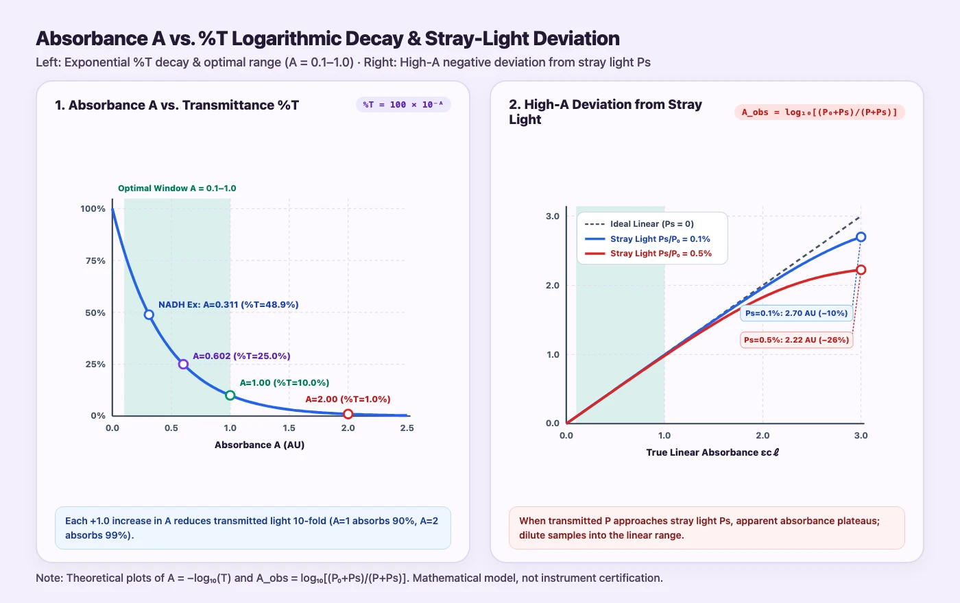
- Converting %T = 25.0% to Absorbance A: Since T = 0.2500, A = 2 − log₁₀(25.0) = 2 − 1.39794 = 0.6021 AU (75.00% of incident light is absorbed; 25.00% is transmitted).
- Applying Dark-Current Subtraction: If blank intensity is I₀ = 1050, sample intensity is I = 290, and dark count is I_dark = 50: Omitting dark subtraction gives 290 ÷ 1050 = 0.2762 (A = 0.5588 AU), underestimating the absorbance by 0.061 AU. For a refresher on base-10 vs. natural logarithms, see the Logarithm Calculation Guide.
Why Does Linearity Break Down Above A > 1.5–2.0? (Stray Light Limit)
At A = 1.0, 10.0% of incident light reaches the detector; at A = 2.0, only 1.0% passes through; at A = 3.0, only 0.1% passes through. When the transmitted signal P becomes very small, a tiny fraction of stray light (P_s) scattered inside the monochromator begins to dominate the denominator. As derived in Chemistry LibreTexts (Wenzel, 1.2: Beer’s Law), the apparent measured absorbance A_obs with stray light P_s is:
For example, if an instrument has a stray light ratio of P_s / P₀ = 0.1% (0.001) and the true linear absorbance of a concentrated sample is εcℓ = 3.0 (so P / P₀ = 0.001):
Even 0.1% stray light causes a 10% negative error at A = 3.0. Combined with high-concentration solute-solute interactions and refractive index changes, this is why analytical protocols recommend diluting samples so that measurements fall within A = 0.1 to 1.0 (%T = 79.4% to 10.0%).
Example 4: 5-Point Linear Calibration Curve (Least Squares) & Unknown Quantification
In quantitative analysis, rather than relying solely on a literature ε value, you measure 3 to 5 standard solutions of known concentration on the same spectrophotometer and fit a least-squares calibration line A = m·c + b.
Below is a 5-point standard dataset (concentration c in mg/L, absorbance A in AU) used to quantify a 5-fold diluted unknown sample (DF = 5) with measured absorbance A_sample = 0.4104 AU:
| Standard # | Concentration c (mg/L) | Measured A (AU) | Fitted  | Residual (A − Â) |
|---|---|---|---|---|
| 1 (Blank) | 0.0 | 0.005 | 0.0054 | −0.0004 |
| 2 | 2.0 | 0.168 | 0.1674 | +0.0006 |
| 3 | 4.0 | 0.329 | 0.3294 | −0.0004 |
| 4 | 6.0 | 0.492 | 0.4914 | +0.0006 |
| 5 | 8.0 | 0.653 | 0.6534 | −0.0004 |
| Mean / Sum | c̄ = 4.0 | Ā = 0.3294 | — | Sum = 0.0000 |
- Sums of squares and cross-products: S_cc = Σ(cᵢ − c̄)² = (−4)² + (−2)² + 0² + 2² + 4² = 40.0 S_cA = Σ(cᵢ − c̄)(Aᵢ − Ā) = 3.2400
- Calibration slope m and intercept b: m = 3.2400 ÷ 40.0 = 0.08100 L/mg b = 0.3294 − 0.08100 × 4.0 = 0.00540 AU Calibration equation: A = 0.08100·c + 0.00540 (R² = 1.0000 [0.999993])
- Back-calculating cuvette concentration of the unknown (A_sample = 0.4104 AU): Because 0.4104 AU lies inside the standard absorbance range (0.005 to 0.653 AU), this is a valid interpolation:
- Undiluted sample concentration c₀ (with DF = 5):
For a detailed derivation of S_xx, S_xy, correlation coefficient r, and R², see the Least Squares Regression Line Guide and the Least Squares Calculator.
How to Reproduce All 4 Examples in the Calculator
Open the Beer-Lambert Law, Absorbance & Calibration Calculator to verify each example in one click:
- Example 1 (NADH 340 nm):
Click the preset “NADH Assay (340nm, ε=6220, c=50μmol/L)”. Tab 1 automatically sets
Target = Absorbance A,ε = 6220,c = 50 μmol/L, andℓ = 1.0 cm, displaying A = 0.3110 AU, %T = 48.87%, and the Optimal Linear Range (0.1 ≤ A ≤ 1.0) badge. - Example 2 (KMnO₄ 10× Dilution & 1 mm Microvolume dsDNA):
Click “KMnO₄ Unknown w/ 10× Dilution (A=0.491, DF=10)” to verify cuvette concentration 200.0000 μmol/L, undiluted stock concentration c₀ = 2000.00 μmol/L, and mass concentration ρ₀ = 316.07 mg/L. Then click “Microvolume dsDNA (260nm, ℓ=1mm, A=0.150)” to switch the path length unit to
mmand confirm 227.2727 μmol/L (75.00 mg/L). - Example 3 (%T and Dark-Corrected Intensity):
Click “Transmittance %T=25% → A=0.6021” to open Tab 2 and verify A = 0.6021 AU. Change the input mode to “From Light Intensities (I₀, I, Dark) → A & %T” and enter
I₀ = 1050,I = 290,I_dark = 50to confirm T = 0.2400 (24.00%) and A = 0.6198 AU. - Example 4 (5-Point Calibration Curve): Click “5-Point Calibration & Unknown (R²=1.0000, DF=5)” to open Tab 3 and verify A = 0.08100·c + 0.00540, R² = 1.0000, cuvette concentration 5.000 mg/L, and undiluted concentration c₀ = 25.00 mg/L (DF = 5×) within the interpolated calibration range.
Use the “Copy Calculation Report (Markdown)” button at the bottom of the tool to paste the complete parameters and results into your lab notebook, and consult the Significant Figures Guide when rounding final reported values.
Common Mistakes & Model Limitations Checklist
- Unit mismatch between c and ε: Always convert mmol/L (× 10⁻³) or μmol/L (× 10⁻⁶) to mol/L when ε is in L/(mol·cm).
- Path length ℓ in microplates and microvolume cells: Standard cuvettes are 1.0 cm, whereas microvolume spectrophotometers use 0.5 mm or 1.0 mm (0.10 cm) and 96-well microplates have meniscus-dependent path lengths that depend on fill volume.
- Extrapolating beyond the highest standard: Never use a linear calibration curve to extrapolate an unknown whose absorbance exceeds your highest standard; dilute the sample with the same buffer/solvent so its absorbance falls inside the calibrated linear range.
- Chemical and instrumental conditions: Molar absorptivity ε depends on wavelength, temperature, solvent, and pH (especially for acid-base indicators, phenols, and proteins). Always zero the instrument with a matched reagent blank.
Frequently Asked Questions (FAQ)
What does a negative absorbance reading (A < 0) mean?
A negative absorbance means the sample transmitted more light to the detector than the blank (I > I₀, or %T > 100%). This typically happens when the blank cuvette had fingerprints, microbubbles, or suspended particles during zeroing, or when the blank solvent did not match the sample matrix. Clean the cuvette, re-zero with a fresh blank, and re-measure.
Should I force the calibration curve through zero (b = 0)?
In routine analytical work using ordinary least squares (A = m·c + b), keeping the fitted intercept b and solving c = (A_sample − b) / m accounts for small cuvette mismatches or reagent blank offsets across the linear range. However, if |b| is unexpectedly large, inspect your blank preparation and check for matrix interference before relying on the curve.
Does doubling percent transmittance (%T) cut absorbance A in half?
No. Because A = 2 − log₁₀(%T) is logarithmic, doubling %T from 25% to 50% decreases absorbance from 0.6021 AU to 0.3010 AU (a change of −log₁₀2 ≈ −0.3010 AU), and doubling %T from 10% to 20% decreases absorbance from 1.0000 AU to 0.6990 AU (again −0.3010 AU). Doubling transmittance always subtracts log₁₀(2) ≈ 0.3010 AU from absorbance.